Linear models: Pushing down and speeding up
R Analytics Blog – 2017 / 10 / 21
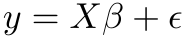
Let’s start with a few observations about linear models. The usual discussion posits a target variable y of
length N and a design matrix X with p columns (of full rank, say) and N rows. The linear model equation can be written
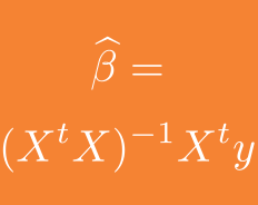
and the least squares solution is obtained by projecting y orthogonally onto the image of X giving the almost iconic formula in the title for the estimated parameters.
The most common case – unless you are a geneticist –
is that X is ‘long’, i.e. we have N >> p. We can test some properties of our least squares solution in this case in a little simulation
p =  1000
N = 10^5
beta = runif(p, -20, 20)

X <- matrix(rnorm(p*N), ncol = p)
y  <- X %*% beta + rnorm(N, sd = 5)

system.time(XtX <- crossprod(X))[3]
## elapsed
## 62.784system.time(Xty <- drop(crossprod(X,y)))[3]## elapsed
## 0.308system.time(beta_est <- solve(XtX, Xty))[3]## elapsed
## 0.355Classical treatments of the least squares solution focus on decomposing X in a suitable manner to address both, the crossproduct and the inversion. This somewhat obscures the fact that there are two distinct data steps:
- a ‘small data’ step: Even with our hypothetical
p = 1000coefficients, the inversion only takes a few seconds - a ‘big data’ step: The crossproduct is what we need to worry about much more for typical large
X!
Chunking and parallelising
Our example case (large X with N >> p) is ideal for chunking and parallelising. Chunking is made easy by packages like
biglm and speedglm that provide the infrastructure for handling chunked data and for updating estimates with new chunks.
Also note that the crossproducts
are ‘embarrassingly parallel’, i.e. they can be calculated via an appropriate ‘lapply’-ification:
library(parallel)

X_chunked <- lapply(split(X, (1:N)%%9) , matrix, ncol = p)

system.time(XtX_chunked <- mclapply(X_chunked, crossprod, mc.cores = 3))[3]
## elapsed
## 31.675XtX2 <- 0; for(xtx in XtX_chunked) XtX2 <- XtX2 + xtx
sum(abs(XtX- XtX2)) ## ~ 0So, chunking and parallelising helps.
To improve things further, one needs to look more closely at the structure of X. One well-known approach is in the MatrixModels-package, which allows to make use of sparsity in X, for instance, when X contains many dummy variables.
Special structures in X – star schema
The situation for which I have not immediately found an adequate package, and which I want to discuss in a bit more detail here, is when X is constructed from some kind of database ‘star schema’. As an example, we can take the fuel price data discussed here.
We start with loading the required packages and by defining a small benchmarking function, which will not only measure execution times, but also give a rough idea on memory usage:
## Clear all -- only if you have saved your other projects
rm(list=ls(all=TRUE))

library(tidyverse)
library(stringr)
library(splines)
library(Matrix)
library(MatrixModels)

## a simple benchmarker
mstest <- function(expr=NULL) {
  mem <- gc(reset = TRUE)[2, c(2,6)]
  st <- proc.time()
  expr
  mem2 <- gc(reset = FALSE)[2, c(2,6)] - mem
  names(mem2) <- c("A_Mem final", "A_Mem max")
  c(A_Time =structure(proc.time()- st, class = "proc_time")[1:3],  mem2)
}
Now load (and clean) the fuel price data (find it on GitHub here). It is a very simple star schema, with fuel prices per station and time as fact table:
pricesAll <- readRDS( "Prices_Demo.rds")%>%
  filter(E10 > 700, E10 < 3500, TimeAggID > 26425,
         ## choose TimeAggID filter to fit to your machine
         !is.na(CompE10))
pricesAll
## StationID TimeAggID E10 CompE10
## <int> <int> <int> <int>
## 1 1 26426 1269 1450
## 2 1 26427 1269 1450
## 3 1 26428 1269 1450
## 4 1 26429 1269 1450
## 5 1 26430 1269 1439
## # ... with 4,859,833 more rowsas well as dimension tables for stations and times:
timesAll <- readRDS( "E_prtimes.rds")
timesAll
## TimeAggID DateHour DateDay HourCl DayCl Brent
## <int> <int> <int> <fctr> <fctr> <int>
## 1 1 14060800 140608 Hour00 Sun 501
## 2 2 14060801 140608 Hour01 Sun 501
## 3 3 14060802 140608 Hour02 Sun 501
## 4 4 14060803 140608 Hour03 Sun 501
## 5 5 14060804 140608 Hour04 Sun 501
## # ... with 27,523 more rowsstationsAll <- readRDS( "C_stationsAll_final.rds")
## add natural splines to stations
NS <- as_data_frame( model.matrix( ~ -1 + ns(lat, df = 3):ns(lng, df = 3),
data = stationsAll ))
names(NS) <- paste0("NS",str_replace_all(names(NS),
"\\:|ns\\(lat, df = \\d+\\)|ns\\(lng, df = \\d+\\)", ""))
stationsAll <- bind_cols(stationsAll, NS)
stationsAll## StationID brandCl lng lat isBAB closeBAB NS11
## <int> <fctr> <dbl> <dbl> <int> <int> <dbl>
## 1 1 Others 10.850848 48.55568 0 0 0.39713860
## 2 2 BfT 10.920224 49.66159 0 0 0.43709986
## 3 3 Others 6.948950 51.16919 0 0 0.01966565
## 4 4 Others 11.451392 48.12189 0 1 0.37167161
## 5 5 Others 12.520820 48.24147 0 0 0.28931168
## # ... with 14,897 more rows, and 8 more variables: NS21 <dbl>, NS31 <dbl>,
## # NS12 <dbl>, NS22 <dbl>, NS32 <dbl>, NS13 <dbl>, NS23 <dbl>, NS33 <dbl>Traditional approach: One big design matrix X
Now, let’s say we want to estimate the influence of
- the brand of the station
- the closeness of the station to a highway (via isBAB, closeBAB)
- the location of the station in Germany (via the natural splines on long / lat)
- the time of day
- the average price of Competitors (CompE10 – I’ll say more about this, later)
etc. on the price of E10 fuel.
In the traditional approach, we join all the dimension information to the fact table and run the model on the resulting large table:
fulldat <- pricesAll %>%
  left_join(select(timesAll, -DateHour, -DateDay )) %>%
  left_join(stationsAll)

object.size(fulldat)/10^6 ## 622MB

RESULT <- NULL

modfor <- as.formula(
  paste0("E10 ~ 1 +  CompE10 + Brent + isBAB + closeBAB + brandCl +",
         "DayCl  +  HourCl +",
         paste(names(NS), collapse = " + ")))

msLM <- mstest(modLM <- lm( modfor, data = fulldat))

RESULT[["trad. LM"]] <- c(msLM, modLM$coefficients)
msLM
## A_Time.user.self A_Time.sys.self A_Time.elapsed A_Mem final
## 41.343 0.854 42.315 2870.500
## A_Mem max
## 5058.200Exploiting the star schema: Lifted matrices
So, how to make this smaller and faster?
The main observation is that the parts of the design matrix, that come from the joined dimension matrices, have a very simple form. For example, when looking at the variables which depend on time only:
matTime = model.Matrix(~ -1 + Brent + DayCl + HourCl, data = timesAll )is the design matrix on the table timesAll and
indTime = as(list(pricesAll$TimeAggID, max(timesAll$TimeAggID)), "indMatrix")is the (sparse version of) the ‘index matrix’, representing the join. This matrix has a 1 in position (ro, co) exactly when TimeAggID[ro] == co and zeros otherwise. It is easy to check that the matrix product of indTime and matTime
is the lift / join of matTime to the fact table
all(indTime %*% matTime == matTime[pricesAll$TimeAggID, ]) ## TRUEThis is a very useful representation, as
- matTime will be comparatively small,
- crossproducts with the index matrix 'indTime' amount to a simple summing over groups, and need to be executed only once, regardless the size of matTime
Furthermore, index matrix algebra is already implemented in the Matrix-package.
Let’s call these objects ‘lifted matrices’. We can actually define them as a simple extension of the classes in Matrix:
setClass("liftMatrix",
         representation(mat = "Matrix",
                        indI  = "indMatrix"))
The beauty of the ‘Matrix’-package (and the S4-system it is built on) is that we now only need to implement the algebra for this new class as a set of S4-methods,
adding to (in one case for the moment: overriding) the existing method-definitions in Matrix:
## changes some 'Matrix'-definitions. Restart R afterwards

setMethod("crossprod", signature( x = "indMatrix", y = "missing"),
          function(x)  Diagonal(x = tabulate(x@perm, x@Dim[2])))

setMethod("crossprod", signature( x = "indMatrix", y = "indMatrix" ),
          function(x, y) {
            l1 <- as(x, "lMatrix")
            l2 <- as(y, "lMatrix")
            crossprod(l1,l2)
            })

setMethod("crossprod", signature( x = "liftMatrix", y = "missing"),
          function(x) crossprod(x@mat, crossprod(crossprod(x@indI) , x@mat)))

setMethod("crossprod", signature( x = "liftMatrix", y = "liftMatrix" ),
          function(x, y)   crossprod(x@mat,
                           crossprod(crossprod(y@indI, x@indI), y@mat)))

setMethod("crossprod", signature( x = "liftMatrix", y = "Matrix" ),
          function(x, y)   {
            crossprod(x@mat, crossprod(x@indI, y)) })

setMethod("crossprod", signature( x = "Matrix", y = "liftMatrix" ),
          function(x, y)   {
            crossprod(x, y@indI) %*% y@mat })
With these definitions, it is now easy to define the ‘lifted’ (or ‘pushed down’, depending on your point of view) version of our fuel price model above, by separately defining the components of the design which stem from the two dimension tables and (for the effect of CompE10) from the fact table itself.
I go through the full calculation here for demonstration purposes. I hope to put this into a more user-friendly format, soon.
msLift <- mstest({

  modforS <- as.formula(
    paste0("~ 1 +  isBAB + closeBAB + brandCl +",
           paste(names(NS), collapse = " + ")))

  XS <- new("liftMatrix",
            mat = model.Matrix(modforS, data = stationsAll )*1.0,
            indI = as(list(pricesAll$StationID, max(stationsAll$StationID)),
                      "indMatrix"))

  modforT <- as.formula(paste0("~ 1 + Brent + DayCl + HourCl"))

  XT <- new("liftMatrix",
            mat = model.Matrix(modforT, data = timesAll )[,-1]*1.0,
            indI = as(list(pricesAll$TimeAggID, max(timesAll$TimeAggID)),
                    "indMatrix"))

  XC  <- Matrix( pricesAll$CompE10, ncol = 1,
                 dimnames = list(NULL, "CompE10"))

  Y <- Matrix(pricesAll$E10, ncol = 1)

  XTXT <- crossprod(XT)
  XSXS <- crossprod(XS)
  XCXC <- crossprod(XC)
  XTXS <- crossprod(XT, XS)
  XTXC <- crossprod(XT, XC)
  XSXC <- crossprod(XS, XC)
  XSY <- crossprod(XS, Y)
  XTY <- crossprod(XT, Y)
  XCY <- crossprod(XC, Y)

  XX <-  rbind(cbind(XTXT, XTXS, XTXC),
               cbind(t(XTXS), XSXS, XSXC),
               cbind(t(XTXC), t(XSXC), XCXC))
  XY <- rbind(XTY, XSY, XCY)

  modLift <- drop(solve(XX, XY))
})

RESULT[["lifted LM"]] <- c(modLift,  msLift)
A bit of arranging of the results for easier comparison:
for(nam in names(RESULT)) RESULT[[nam]]<-
  data.frame( estimate = RESULT[[nam]]) %>%
  rownames_to_column(var = "term") %>%
  mutate(model = nam)

resultWide <- bind_rows(RESULT) %>% dplyr::select(model, term, estimate) %>%
  spread(model, estimate)

head(resultWide, 10)
## term lifted LM trad. LM
## 1 A_Mem final 84.000000 2870.500000
## 2 A_Mem max 2103.000000 5058.200000
## 3 A_Time.elapsed 3.510000 42.315000
## 4 A_Time.sys.self 0.204000 0.854000
## 5 A_Time.user.self 3.291000 41.343000
## 6 brandClAral 23.329966 23.329966
## 7 brandClAvia -5.360235 -5.360235
## 8 brandClBfT -17.300784 -17.300784
## 9 brandClEsso -3.675214 -3.675214
## 10 brandClHEM -20.194030 -20.194030Four seconds instead of forty – Pretty impressive, huh?
Well, of course, I have massaged the example a bit. The model we have been looking at is a pretty extreme case. Almost all the explanatory variables are ‘lifts’ from one of the dimension tables. So the model is almost a product of two completely separate models. I actually had to sneak in the variable ‘CompE10’ (with all the problems, endogeneity, inconsistency, this variable brings, were we to really try to interpret this model) in order to make the example a truly non-product one.
Still, this approach is worthwile in many cases, and I will soon publish a more elaborate example, including how to deal with chunked and partitioned data, as well as allowing fixed effects.
So stay tuned!